Two years ago, I started to study Computational Optimal Transport (OT), and, now, it is time to wrap up informally the main ideas by using an Operations Research (OR) perspective with a Machine Learning (ML) motivation.

Yes, an OR perspective.

Why an OR perspective?

Well, because most of the current theoretical works on Optimal Transport have a strong functional analysis bias, and, hence, the are pretty far to be an “easy reading” for anyone working on a different research area. Since I’m more comfortable with “summations” than with “integrations”, in this post I focus only on Discrete Optimal Transport and on Kantorovich-Wasserstein distances between a pair of discrete measures.

Why an ML motivation?

Because measuring the similarity between complex objects is a crucial basic step in several #machinelearning tasks. Mathematically, in order to measure the similarity (or dissimilarity) between two objects we need a metric, i.e., a distance function. And Optimal Transport gives us a powerful similarity measure based on the solution of a Combinatorial Optimization problem, which can be formulated and solved with Linear Programming.

The main Inspirations for this post are:

• My current favorite tutorial is Optimal Transport on Discrete Domains, by Justin Solomon.
• Two years ago, I started to study this topic thanks to Giuseppe Savaré, and I wrote this post by looking also to his set of slides. He has several interesting papers and you can look at his publications list.
• For a complete overview of this topic look at the Computational Optimal Transport book, by Gabriel Peyré and Marco Cuturi. These two researchers, together with Justin Solomon, where among the organizers of two #NeurIPS workshops, in 2014 and in 2017, on Optimal Transport and Machine Learning.
• For a broader history of Combinatorial Optimization till 1960, see this manuscript by Alexander Schrijver.

DISCLAIMER 1: This is a long “ongoing” post, and, despite my efforts, it might contain errors of any type. If you have any suggestion for improving this post, please (!), let me know about: I will be more than happy to mention you (or any of your avatars) in the acknowledgement section. Otherwise, if you prefer, I can offer you a drink, whenever we will meet in real life.

DISCLAIMER 2: I wrote this post while reading the book Ready Player One, by Ernest Cline.

DISCLAIMER 3: I’m recruiting postdocs. If you like the topic of this post and you are looking for a postdoc position, write me an email.

Similarity measures and distance functions

A metric is a function, usually denoted by $d$, between a pair of objects belonging to a space $X$:

Given any triple of points $x,y,z \in X$, the conditions that $d$ must satisfy in order to be a metric are:

1. $d(x,y) \geq 0$ (non negativity)
2. $d(x,y) = 0 \Leftrightarrow x=y$ (identity of indiscernibles)
3. $d(x,y) = d(y,x)$ (symmetry)
4. $d(x,z) \leq d(x,y) + d(y,z)$ (triangle inequality or subadditivity)

If the space $X$ is $\mathbb{R}^k$, then $\mathbf{x}, \mathbf{y}, \mathbf{z}$ are vectors of $k$ elements, and the most common distance is indeed the Euclidean function

where $x_i$ is the $i$-th component of the vector $\mathbf{x}$. Clearly, the algorithmic complexity of computing (in finite precision) this distance is linear with the dimension of $X$.

QUESTION: What if we want to compute the distance between a pair of clouds of $n$ points defined in $\mathbb{R}^k$?

If we want to compute the distance between the two vectors, that represent the two clouds of $n$ points, we need to define a distance function.

Let me fix the notation first. If $\mathbf{x}$ is a vector, then $x_i$ is the $i$-th element. Suppose we have two matrices $\mathbf{X}$ and $\mathbf{Y}$ with $n \times k$ elements, which represent $n$ points in $\mathbb{R}^k$. We denote by $\mathbf{x}_i$ the $i$-th row of matrix $\mathbf{X}$, and by $x_{ij}$ the $j$-th element of row $i$. Indeed, the rows $\mathbf{x}_i$ and $\mathbf{y}_i$ of the two matrices give the coordinates $x_{i1},\dots,x_{ik}$ and $y_{i1},\dots,y_{ik}$ of the two corresponding points.

Whenever $k=1$, a simple choice is to consider the Minkowski Distance, which is a metric for normed vector spaces:

where typical values of $p$ are:

• $p=1$ (Manhattan distance)
• $p=2$ (Euclidean distance, see above)
• $p=\infty$ (Infinity distance)

We have also the Minkowski norm, that is a function

computed as

Whenever $k>1$, we have to consider a more general distance function:

such that the relations (1)-(4) are satisfied. We could use as distance function $D(\mathbf{X},\mathbf{Y})$ any matrix norm, but, to begin with, we can use the Minkowski distance twice in cascade as follows.

1. First, we compute the distance between a pair of points in $\mathbb{R}^k$, which we call the ground distance, using $M_q$, with $q\geq 1$. By applying this function to all the $n$ pairs of points, we get a vector $\mathbf{z}$ of $n$ non-negative values:

1. Second, we apply the Minkowski norm $\ell_p$ to the vector $\mathbf{z}$.

Composing these two operations, we can define a distance function between a pair of vectors of points (i.e., pair of matrices) as follows:

Note that for $p=q=2$, we get

which is the Frobenius Norm of the element wise difference $\mathbf{X} - \mathbf{Y}$.

The main drawback of this distance function is that it implicitly relies on the order (position) of the single points in the two input vectors: any permutation of one (or both) of the two vectors will yield a different value of the ground distance. This happens because the distance function between the two input vectors considers only “interactions” between the $i$-th pair of points stored at the same $i$-th position in the two vectors.

IMPORTANT. Here is where Discrete Optimal Transport comes into action: it offers an alternative distance function based on the solution of a Combinatorial Optimization problem, which is, in the simplest case, formulated as the following Linear Program:

If you have a minimal #orms background at this point you should have recognized that this problem is a standard Assignment Problem: we have to assign each point of the first vector $\mathbf{x}$ to a single point of the second vector $\mathbf{y}$, in such a way that the overall cost is minimum. From an optimal solution of this problem, we can select among all possible permutations of the rows of $\mathbf{Y}$, the permutation that gives the minimal value of the Frobenius norm.

Whenever the ground distance $d(\mathbf{x},\mathbf{y})$ is a metric, then $\mathcal{W}_d(\mathbf{X},\mathbf{Y})$ is a metric as well. In other terms, the optimal value of this problem is a measure of distance between the two vectors, while the optimal values of the decision variables $\mathbf{\pi}$ gives a mapping from the rows of $\mathbf{X}$ to the rows of $\mathbf{Y}$ (in OT terminology, an optimal plan). This is possible because the LP problem has a Totally Unimodular coefficient matrix, and, hence, every basic optimal solution of the LP problem has integer values.

WAIT, LET ME STOP HERE FOR A SECOND!

I am being too technical, too early. Let me take a step back in History.

Once Upon a Time: from Monge to Kantorovich

The History of Optimal Transport is quite fascinating and it begins with the Mémoire sur la théorie des déblais et des remblais by Gaspard Monge (1746-1818). I like to think of Gaspard as visiting the Dune of Pilat, near Bordeaux, and then writing his Mémoire while going back to home… but this is only my imagination. Still, particles of sand give me the most concrete idea for passing from a continuous to a discrete problem.

In his Mémoire, Gaspard Monge considered the problem of transporting “des terres d’un lieu dans un autre” at minimal cost. The idea is that we have first to consider the cost of transporting a single molecule of “terre”, which is proportional to its weight and to the distance from its initial and final position. The total cost of transportation is given by summing up the transportation cost of each single molecule. Using the Lex Schrijver’s words, Monge’s transportation problem was camouflaged as a continuous problem.

The idea of Gaspard is to assign to each initial position a single final destination: it is not possible to split a molecule into smaller parts. This unsplittable version of the problem posed a very challenging problem where “the direct methods of the calculus of variations fail spectacularly” (Lawrence C. Evans, see link at page 5). This challenge stayed unsolved until the work of Leonid Kantorovich (1912-1986).

Curiously, Leonid did not arrive to the transportation problem while studying directly the work of Monge. Instead, he was asked to solve an industrial resource allocation problem, which is more general than Monge’s problem. Only a few years later, he reconsidered his contribution in terms of the continuous probabilistic version of Monge’s transportation problem. However, I am unable to state the true technical contributions of Leonid with respect to the work of Gaspard in a short post (well, honestly, I would be unable even in an infinite post), but I recommend you to read the Long History of the Monge-Kantorovich Transportation Problem.

Anyway, I have pretty clear the two main concepts that are the foundations of the work by Kantorovich:

1. RELAXATION: He relaxes the problem posed by Gaspard and he proves that an optimal solution of the relaxation equals an optimal solution of the original problem (Here is the link to the very unofficial soundtrack of his work: “Relax, take it easy!”). Indeed, Leonid relaxed formulation allows each molecule to be split across several destinations, differently from the formulation of Monge. In OR terms, he solves a Hitchcock Problem, not an Assignment Problem. For more details, see Chapter 1 of the Computational Optimal Transport.

1. DUALITY: Leonid uses a dual formulation of the relaxed problem. Indeed, he invented the dual potential functions and he sketched the first version of dual simplex algorithm. Unfortunately, I studied Linear Programming duality without having an historical perspective, and hence duality looks like obvious, but at the time is was clearly a new concept.

For the records, Leonid Kantorovich won the Nobel Prize, and his autobiography merits to be read more than once.

Well, I have still so much to learn from the past!

Two Fields medal winners: Alessio Figalli and Cedric Villani

If you think that Optimal Transport belongs to the past, you are wrong!

Last summer (2018), in Rio de Janeiro, Alessio Figalli won the Fields Medal with this citation:

“for his contributions to the theory of optimal transport, and its application to partial differential equations, metric geometry, and probability”

Alessio is not the first Fields medalist who worked on Optimal Transport. Already Cedric Villani, who wrote the most cited book on Optimal Transport [1], won the Fields Medal in 2010. I strongly suggest you to look any of his lectures available on Youtube. And … do you know that Villani spent a short period of time during his PhD in my current Math Dept. at University of Pavia?

As an extra bonus, if you don’t know what a Fields Medal is, you can have Robin Williams to explain the prize in this clip taken from Good Will Hunting.

Discrete Optimal Transport and Linear Programming

It is time of being technical again and to move from the Monge assignment problem, to the Kantorovich “relaxed” transportation problem. In the assignment model presented above, we are implicitly considering that all the positions are occupied by a single molecule of unitary weight. If we want to consider the more general setting of Discrete Optimal Transport, we need to consider the “mass” of each molecule, and to formulate the problem of transporting the total mass at minimum cost. Before presenting the model, we define formally the concept of a discrete measure and of the cost matrix between all pairs of molecule positions.

DISCRETE MEASURES: Given a of vector of $n$ positions $\mathbf{x}_i$, and given the Dirac delta function, we can define the Dirac measures $\delta_{\mathbf{x}_i}$ as

Given a vector of $n$ weights $\mu_i$, one associated to each element of $\mathbf{x}$, we can define the discrete measure $\mathbf{\mu}$ as

Note the $\mu$ is a function of type: $\mu : A \rightarrow \mathbb{R}_+$, for any subset $A$ of $X$. The vector $\mathbf{x}$ is called the support of the measure $\mathbf{\mu}$. In Computer Science terms, a discrete measure is defined by a vector of pairs, where each pair contains a positive number $\mu_i$ (the measured value) and its support point $\mathbf{x}_i$ (the location where the measure occurred). Note that $\mathbf{x}_i$ is a (small?) vector storing the coordinates of the $i$-th point.

COST MATRIX: Given two discrete measures $\mathbf{\mu}$ and $\mathbf{\nu}$, the first with support $\mathbf{x}$ and the second with support $\mathbf{y}$, we can define the following cost matrix:

where $d$ is a distance function, such as, for instance, the Minkowski distance $M_q(\mathbf{x},\mathbf{y})$ defined before. Note that $\mathbf{\mu}$ has $n$ elements, and $\mathbf{\nu}$ has $m$ elements.

Kantorovich-Wasserstein distances between two discrete measures

At this point, we have all the basic elements to define the Kantorovich-Wasserstein distance function between discrete measures in terms of the solution of a (huge) Linear Program.

INPUT: Two discrete measures $\mathbf{\mu}$ and $\mathbf{\nu}$ defined on a metric space $X$, and the corresponding supports $\mathbf{x}$ and $\mathbf{y}$, having $n$ and $m$ elements, respectively. A distance function $d$, which permits to compute the cost $c_{ij}$.

OUTPUT: A transportation plan $\mathbf{\pi}$ and a value of distance of $\mathcal{W}(\mathbf{\mu}, \mathbf{\nu})$ that corresponds to an optimal solution of the following Linear Program:

This Linear Program is indeed a special case of the Transportation Problem, known also as the Hitchcock-Koopmans problem. It is a special case because the cost vector has a strong structure that should be exploited as much as possible.

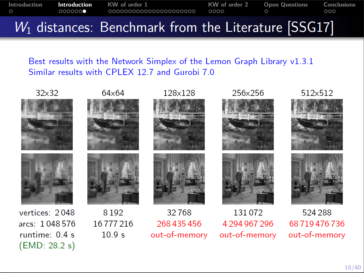
Computational Challenge: While the previous problem is polynomially solvable, the size of practical instances is very large. For instance, if you want to compute the distance between a pair of grey scale images of resolution $512 \times 512$ pixels, you end up with an LP with $512^4 = 68\;719\;476\;736$ cost coefficients. Hence, these problems must be handled with care. If you want to see how the solution time and memory requirement scale for grey scale image, please, have a look at the slides of my talk at Aussois (2018).

KANTOROVICH-WASSERSTEIN DISTANCE

Whenever

1. The two measure are discrete probability measures, that is, both $\sum_{i=1}^n \mu_i = 1$ and $\sum_{j = 1}^m \nu_j = 1$ (i.e., $\mathbf{\mu}$ and $\mathbf{\nu}$ belongs to the probability simplex), and,
2. The cost vector is defined as the $p$-th power of a distance,

then we define the Kantorovich-Wasserstein distance of order $p$ as the following functional:

where the set $U$ is defined as:

From a mathematical perspective, the most interesting case is the order $p=2$, which generalizes the Euclidean distance to discrete probability vectors. Note that in this formulation, the two constraint sets defining $U$ could be replaced with equality constraints, since $\mathbf{\mu}$ and $\mathbf{\nu}$ belongs to the probability simplex. In addition, any Combinatorial Optimization algorithm must be used with care, since all the cost and constraint coefficients are not integer. Note: The $p$ power used for the ground distance must not be confused with the order (power) of a Kantorovich-Wasserstein distance.

EARTH MOVER DISTANCE

A particular case of the Kantorovich-Wasserstein distance very popular in the Computer Vision research community, is the so-called Earth Mover Distance (EMD) [2], which is used between a pair of $k$-dimensional histograms obtained by preprocessing the images of interest. In this case, (i) we have $n=m$, (ii) we do not require the discrete measures to belong to the probability simplex, and (iii) we do not even require that the two measures are balanced, that is, $\sum_{i=1}^n \mu_i = \sum_{j=1}^n \nu_j$. In Optimal Transport terminology, the Earth Mover Distance solves an unbalanced optimal transport problem. For the EMD, the feasibility set $U$ is replaced by the set:

The cost function is taken with the order $p=1$:

The most used function $d$ is the Minkowski distance induced by the $\ell_p$ norm.

WORD MOVER DISTANCE

A very interesting application of discrete optimal transport is the definition of a metric for text documents [3]. The main idea is, first, to exploit a word embedding obtained, for instance, with the popular word2vec neural network [4], and, second, to formulate the problem of “transporting” a text document into another at minimal cost.

Yes, but … how we compute the ground distance between two words?

A word embedding associates to each word of a given vocabulary a vector of $\mathbb{R}^k$. For the pre-trained embedding made available by Google at this archive, which contains the embedding of around 3 millions of words, $k$ is equals to 300. Indeed, given a vocabulary of $n$ words and fixed a dimension $k$, a word embedding is given by a matrix $\mathbf{X}$ of dimension $n \times k$: Row $\mathbf{x}_i$ gives the $k$-dimensional vector representing the word embedding of word $i$.

In this case, instead of having discrete measures, we deal with normalized bag-of-words (nBOW), which are vector of $\mathbb{R}^n$, where $n$ denotes the number of words in the vocabulary. If a text document $\mathbf{\mu} \in \mathbb{R}^n$ contains $t_i$ times the word $i$, then $\mathbf{\mu}_i = \frac{t_i}{\sum_{j=1}^n t_j}$. At this point is clear that the ground distance between a pair of words is given by the distance between the corresponding embedding vectors in $\mathbb{R}^k$, that is, given two words $i$ and $j$, then

Finally, given two text documents $\mathbf{\mu}$ and $\mathbf{\nu}$, we can formulate the Linear Program that gives the Word Mover Distance as:

where the set $U$ is defined as:

If you are serious reader, and you are still reading this post, then it is clear that the Word Mover Distance is exactly a Kantorovich-Wasserstein distance of order 1, with an Euclidean ground distance. If you are interested in the quality of this distance when used within a nearest neighbor heuristic for a text classification task, we refer to [3]. (While writing this post, I started to wonder how would perform a WMD of order 2, but this is another story…)

Interesting Research Directions

The following are the research topics I am interested in right now. Each topic deserves its own blog post, but let me write here just a short sketch.

• Computational Challenges: The development of efficient algorithms for the solution of Optimal Transport problems is an active area of research. Currently, the preferred (heuristic) approach is based on so-called regularized optimal transport, introduced originally in [5]. Indeed, regularized optimal transport deserves its own blog post. In two recent works, together with my co-authors, we tried to revive the Network Simplex for two special cases: Kantorovich-Wasserstein distances of order 1 for $k$-dimensional histograms [6] and Kantorovich-Wasserstein distances of order 2 for decomposable cost functions [7]. The second paper was presented as a poster at NeurIPS2018. (If you ever read any of the two papers, please, let me know what you think about them)

• Unbalanced Optimal Transport: The computation of Kantorovich-Wasserstein distance for pair of unbalanced discrete measures is very challenging. Last year, a brilliant math student finished a nice project on this topic, which I hope to finalize during the next semester.

• Barycenters of Discrete Measures: The Kantorovich-Wasserstein distance can be used to generalize the concept of barycenters, that is, the problem of finding a discrete measure that is the closest (in Kantorovich terms) to a given set of discrete measures. The problem of finding the barycenter can be formulated as a Linear Program, where the unknowns (the decision variables) are both the transport plan and the discrete measure representing the barycenter. For instance, the following images, taken from our last draft paper, represents the barycenters of each of the 10 digits of the MNIST data set of handwritten images (each image is the barycenter of other $3\;200$ images).

• Distances between Discrete Measures defined on different metric spaces: This topic is at the top of my 2019 resolutions. There are a few papers by Facundo Mémoli on this topic, which are based on the so-called Gromov-Wasserstein distance and that requires the solution of a Quadratic Assignment Problem (QAP).

Now, it’s time to close this post with final remarks.

Optimal Transport: A brilliant future?

Given the number and the quality of results achieved on the Theory of Optimal Transport by “pure” mathematicians, it is the time to turn these theoretical results into a set of useful algorithms implemented in efficient and scalable solvers. So far, the only public library I am aware of is POT: Python Optimal Transport.

On Medium, C.E. Perez claims that Optimal Transport Theory (is) the New Math for Deep Learning. In his short post, he explains how Optimal Transport is used in Deep Learning algorithms, specifically in Generative Adversarial Networks (GANs), to replace the Kullback-Leibler (KL) divergence.

Honestly, I do not have a clear idea regarding the potential impact of Kantorovich distances on GANs and Deep Learning in general, but I think there are a lot of research opportunities for everyone with a strong passion for Computational Combinatorial Optimization.

And you, what do you think about the topics presented in this post?

As usual, I will be very happy to hear from you, in the meantime…

GAME OVER

Acknowledgement

I would like to thank Marco Chiarandini, Stefano Coniglio, and Federico Bassetti for constructive criticism of this blog post.

References

1. Villani, C. Optimal transport, old and new. Grundlehren der mathematischen Wissenschaften, Vol.338, Springer-Verlag, 2009. [pdf]

2. Rubner, Y., Tomasi, C. and Guibas, L.J., 2000. The earth mover’s distance as a metric for image retrieval. International journal of computer vision, 40(2), pp.99-121. [pdf]

3. Kusner, M.J., Sun, Y., Kolkin, N.I., Weinberger, K.Q. From Word Embeddings To Document Distances. Proceedings of the 32 nd International Conference on Machine Learning, Lille, France, 2015. [pdf]

4. Mikolov, T., Sutskever, I., Chen, K., Corrado, G.S. and Dean, J., 2013. Distributed representations of words and phrases and their compositionality. In Advances in neural information processing systems (pp. 3111-3119). [pdf]

5. Cuturi, M., 2013. Sinkhorn distances: Lightspeed computation of optimal transport. In Advances in neural information processing systems (pp. 2292-2300). [pdf]

6. Bassetti, F., Gualandi, S. and Veneroni, M., 2018. On the Computation of Kantorovich-Wasserstein Distances between 2D-Histograms by Uncapacitated Minimum Cost Flows. arXiv preprint arXiv:1804.00445. [pdf]

7. Auricchio, G., Bassetti, F., Gualandi, S. and Veneroni, M., 2018. Computing Kantorovich-Wasserstein Distances on d-dimensional histograms using (d+1)-partite graphs. NeurIPS, 2018.[pdf]

This morning, after reading this very nice post, I decided to challenge myself in Python and to have a look at the impact of mispredicted branches in a language different from C/C++. The basic idea was to use only Python builtins: external libraries are not allowed!

As a benchmark, I grabbed a large text file from P. Norvig’s website, which is 6’488’666 byte long.

The final answer? Yes, mispredicted branches have a huge impact in Python too.

The hidden answer? Python dictionaries ever stop to surprise me: they are REALLY efficient.

NOTE: The followig code snippets were executed in a Python 3.5 notebook, on a windows machine, running Windows 10 and Anaconda Python 3.5 64 bits. You can find my notebook on my Blog GitHub repo. Don’t ask me why, but this blog entry is better visualized directly on GitHub.

UPDATE: Well, most of the time I would use my first implementation based on the filter builtin function, and I would try for alternative implementations only after a profiler has shown that removing blanks is a true bottleneck of my whole program. As written in the title, this post is meant as a basic exercise in Python.

First attempt: Functional style

In Python, I prefer to write as much code in functional style as possible, relying on the 3 basic functions:

1. map
2. filter
3. reduce (this is in the functools module and it is not a true builtin)

Therefore, after few preliminaries, here is my first code snippet:

1
2
3
4
5
6
7
8
9
10
11
12
13
14
15

import cProfile

# Download file from: 'http://norvig.com/big.txt'
big = open('big.txt', 'r')

# Read the while file
test = big.read()

def RemoveBlanksFilter(in_str):
    result = filter(lambda c: c != '\r' and c != '\t' and c != ' ', in_str)
    return "".join(result)

test_result = RemoveBlanksFilter(test)

cProfile.run('RemoveBlanksFilter(test)')

         6488671 function calls in 1.956 seconds

   Ordered by: standard name

   ncalls  tottime  percall  cumtime  percall filename:lineno(function)
        1    0.000    0.000    1.955    1.955 <ipython-input-3-eeb7d3495697>:1(RemoveBlanksFilter)
  6488666    0.870    0.000    0.870    0.000 <ipython-input-3-eeb7d3495697>:2(<lambda>)
        1    0.000    0.000    1.956    1.956 <string>:1(<module>)
        1    0.000    0.000    1.956    1.956 {built-in method builtins.exec}
        1    0.000    0.000    0.000    0.000 {method 'disable' of '_lsprof.Profiler' objects}
        1    1.085    1.085    1.955    1.955 {method 'join' of 'str' objects}

Wow, I didn’t realize that I would have call the lambda function for every single byte of my input file. This is clearly too much overhead.

2nd attempt: remove function calls overhead

Let me drop my functional style, and write a plain old for-loop:

1
2
3
4
5
6
7
8

def RemoveBlanks(in_str):
    result = []
    for c in in_str:
        if c != '\r' and c != '\t' and c != ' ':
            result.append(c)
    return "".join(result)

print('Is test passed:', test_result == RemoveBlanks(test))

Is test passed: True

1

cProfile.run('RemoveBlanks(test)')

         5452148 function calls in 1.566 seconds

   Ordered by: standard name

   ncalls  tottime  percall  cumtime  percall filename:lineno(function)
        1    1.210    1.210    1.553    1.553 <ipython-input-6-5e45e3056bc2>:1(RemoveBlanks)
        1    0.012    0.012    1.566    1.566 <string>:1(<module>)
        1    0.000    0.000    1.566    1.566 {built-in method builtins.exec}
  5452143    0.310    0.000    0.310    0.000 {method 'append' of 'list' objects}
        1    0.000    0.000    0.000    0.000 {method 'disable' of '_lsprof.Profiler' objects}
        1    0.033    0.033    0.033    0.033 {method 'join' of 'str' objects}

Mmm… we just shift the problem to the list append function calls. Maybe we can do better by working in place.

3rd attempt: work in place

Well, almost in place: Python string are immutable; therefore, we first copy the string into a list, and then we work in place over the copied list.

1
2
3
4
5
6
7
8
9
10

def RemoveBlanksInPlace(in_str):
    buffer = list(in_str)
    pos = 0
    for c in in_str:
        if c != '\r' and c != '\t' and c != ' ':
            buffer[pos] = c
            pos += 1
    return "".join(buffer[:pos])

print('Is test passed:', test_result == RemoveBlanksInPlace(test))

Is test passed: True

1

cProfile.run('RemoveBlanksInPlace(test)')

         5 function calls in 1.158 seconds

   Ordered by: standard name

   ncalls  tottime  percall  cumtime  percall filename:lineno(function)
        1    1.113    1.113    1.145    1.145 <ipython-input-9-99d36ae6359e>:1(RemoveBlanksInPlace)
        1    0.013    0.013    1.158    1.158 <string>:1(<module>)
        1    0.000    0.000    1.158    1.158 {built-in method builtins.exec}
        1    0.000    0.000    0.000    0.000 {method 'disable' of '_lsprof.Profiler' objects}
        1    0.032    0.032    0.032    0.032 {method 'join' of 'str' objects}

Ok, working in place does have an impact. Let me go on the true point: avoiding mispredicted branches.

4th attempt: to avoid mispredicted branches

As in the original blog post:

1
2
3
4
5
6
7
8
9
10
11
12
13
14
15
16
17
18
19
20

def RemoveBlanksNoBranch(in_str):
    # Build table
    table = []
    for ic in range(256):
        c = chr(ic)
        if c == '\r' or c == '\t' or c == ' ':
            table.append(0)
        else:
            table.append(1)

    # Removal
    buffer = list(in_str)
    pos = 0
    for c in in_str:
        buffer[pos] = c
        pos += table[ord(c)]  # ord() is a function --> bottleneck
    return "".join(buffer[:pos])


print('Is test passed:', test_result == RemoveBlanksNoBranch(test))

Is test passed: True

1

cProfile.run('RemoveBlanksNoBranch(test)')

         6489183 function calls in 1.474 seconds

   Ordered by: standard name

   ncalls  tottime  percall  cumtime  percall filename:lineno(function)
        1    1.235    1.235    1.460    1.460 <ipython-input-12-1bd75a3de21d>:1(RemoveBlanksNoBranch)
        1    0.014    0.014    1.474    1.474 <string>:1(<module>)
      256    0.000    0.000    0.000    0.000 {built-in method builtins.chr}
        1    0.000    0.000    1.474    1.474 {built-in method builtins.exec}
  6488666    0.192    0.000    0.192    0.000 {built-in method builtins.ord}
      256    0.000    0.000    0.000    0.000 {method 'append' of 'list' objects}
        1    0.000    0.000    0.000    0.000 {method 'disable' of '_lsprof.Profiler' objects}
        1    0.033    0.033    0.033    0.033 {method 'join' of 'str' objects}

Ouch!!! These are getting even worse! Why? Well, ‘ord’ is a function, so we are getting back the overhead of function calls. Can we do better by using a dictionary instead of an array?

5th attempt: use a dictionary

Let me use a dictionary in order to avoid the ‘ord’ function calls.

1
2
3
4
5
6
7
8
9
10
11
12
13
14
15
16
17
18
19
20
21
22
23

def RemoveBlanksNoBranchDict(in_str):
    if type(in_str) != str:
        raise TypeError('This function works only for strings')

    # Build table
    table = {}
    for ic in range(256):
        c = chr(ic)
        if c == '\r' or c == '\t' or c == ' ':
            table[c] = 0
        else:
            table[c] = 1

    # Removal
    buffer = list(in_str)
    pos = 0
    for c in in_str:
        buffer[pos] = c
        pos += table[c]
    return "".join(buffer[:pos])


print('Is test passed:', test_result == RemoveBlanksNoBranchDict(test))

Is test passed: True

1

cProfile.run('RemoveBlanksNoBranchDict(test)')

         261 function calls in 0.771 seconds

   Ordered by: standard name

   ncalls  tottime  percall  cumtime  percall filename:lineno(function)
        1    0.724    0.724    0.758    0.758 <ipython-input-15-46ad4c3f0b26>:1(RemoveBlanksNoBranchDict)
        1    0.013    0.013    0.771    0.771 <string>:1(<module>)
      256    0.000    0.000    0.000    0.000 {built-in method builtins.chr}
        1    0.000    0.000    0.771    0.771 {built-in method builtins.exec}
        1    0.000    0.000    0.000    0.000 {method 'disable' of '_lsprof.Profiler' objects}
        1    0.034    0.034    0.034    0.034 {method 'join' of 'str' objects}

Oooh, yes! Now we can see that without mispredicted branches we can really speed up our algorithm.

Is this the best pythonic solution? No, surely not, but still it is an interesting remark to keep in mind when coding.

Final remark: a simple pythonic solution

Likely, the simplest pythonic solution is just to use the ‘replace’ string function as follows:

1
2
3
4
5
6
7

def RemoveBlanksBuiltin(in_str):
    s1 = in_str.replace('\r','')
    s2 = s1.replace('\t','')
    return s2.replace(' ','')


print('Is test passed:', test_result == RemoveBlanksBuiltin(test))

Is test passed: True

1

cProfile.run('RemoveBlanksBuiltin(test)')

         7 function calls in 0.065 seconds

   Ordered by: standard name

   ncalls  tottime  percall  cumtime  percall filename:lineno(function)
        1    0.001    0.001    0.064    0.064 <ipython-input-18-58fd6655cfba>:1(RemoveBlanksBuiltin)
        1    0.001    0.001    0.065    0.065 <string>:1(<module>)
        1    0.000    0.000    0.065    0.065 {built-in method builtins.exec}
        1    0.000    0.000    0.000    0.000 {method 'disable' of '_lsprof.Profiler' objects}
        3    0.063    0.021    0.063    0.021 {method 'replace' of 'str' objects}

Here we are, the best solution is indeed to use a builtin function, whenever it is possible, even if this was not the real aim of this exercise.

Please, let me know if you have some comments or a different solution in Python.

In this post, I like to share a simple idea on how to solve to optimality some hard instances of the Graph Coloring problem. This simple idea yields a “new time” record for a couple of hard instances.

To date, the best exact approach to solve Graph Coloring is based on Branch-and-Price [1, 2, 3]. The branch-and-price method is completely different from the Constraint Programming approach I discussed in a previous post. A key component of Branch-and-Price is the column generation phase, which is intuitively quite simple, but mathematically rather involved for a short blog post.

Here, I want to show you that a modern Mixed Integer Programming (MIP) solver, such as Gurobi or CPLEX, can solve a few hard instances of graph coloring with the following “null implementation effort”:

1. Enumerate all possible columns
2. Build a .mps instance with those columns
3. Use a MIP solver to solve the .mps instance

Indeed, in this post we try to answer to the following question:

Is there any hope to solve any hard graph coloring instances with this naive approach?

Formulation

Given an undirected graph $G=(V,E)$ and a set of colors $K$, the minimum (vertex) graph coloring problem consists of assigning a color to each vertex, while every pair of adjacent vertices gets a different color. The objective is to minimize the number of colors used in a solution.

The branch-and-price approach to graph coloring is based on a set covering formulation. Let $S$ be the collection of all the maximal stable sets of $G$, and let $S_i \subseteq S$ be the maximal stable sets that contain the vertex $i$. Let $\lambda_s$ be a 0-1 variable equal to 1 if all the vertices in the maximal stable set $s \in S$ get assigned the same color. Hence, the set covering model is:

Indeed, we “cover” every vertex of $G$ with the minimal number of maximal stable sets. The issue with this model is the total number of maximal stable sets in $G$, which is exponential in the number of vertices of G.

Column Generation is a “mathematically elegant” method to by-pass this issue: it lets you to solve the set covering model by generating a very small subset of the elements in $S$. This happens by repeatedly solving an auxiliary problem, called the pricing subproblem. For graph coloring, the pricing subproblem consists of a Maximum Weighted Stable Set problem. If you are interested in Column Generation, I recommend you to look at the first chapter of the Column Generation book, which contains a nice tutorial on the topic, and I would strongly recommend reading the nice survey “Selected Topics in Column Generation”, [4].

How many maximal stable sets are in a hard graph coloring instance?

If this number were not so high, we could enumerate all the stable sets in $S$ and attempt to directly solve the set covering model without resorting to column generation. However, “high” is a subjective measure, so let me do some computations on my laptop and give you some precise numbers.

Hard instances

Among the DIMACS instances of Graph Coloring, there are a few instances proposed by David Johnson, which are still unsolved (in the sense that we have not a computational proof of optimality of the best known upper bounds).

The table below shows the dimensions of these instances. The name of instances are DSJC{n}.{d}, where {n} is the number of vertices and {d} gives the density of the graph (e.g., DSJC125.9 has 125 vertices and 0.9 of density).

As you can see the number of maximal stable sets (i.e. the cardinality of $S$) of several instances is not so high, above all for very dense graphs, where the number of stables set is less than the number of edges. However, for sparse graphs, the number of maximal stable sets is too large for the memory available in my laptop.

Now, let me re-state the main question of this post:

Can we enumerate all the maximal stable sets of $G$ and use a MIP solver such as Gurobi or CPLEX to solve any Johnson’s instance of Graph Coloring?

Results

I have written a small script which uses Cliquer to enumerate all the maximal stable sets of a graph, and then I generate an .mps instance for each of the DSJC instance where I was able to store all maximal stable sets. The .mps file are on my public GitHub repository for this post.

The table below shows some numbers for the sparse instances obtained using Gurobi (v6.0.0) with a timeout of 10 minutes on my laptop. If you compare these numbers with the results published in the literature, you can see that they are not bad at all.

Believe me, these number are not bad at all, and establish a new TIME RECORD.

For example, the instance DSJC250.9 was solved to optimality only recently in 11094 seconds by [3], while the column enumeration approach solves the same instance on a similar hardware in only 23 seconds (!), and, honestly, our work in [2] did not solve this instance to optimality at all.

Can we ever solve to optimality DSJC500.9 and DSJC1000.9 via Column Enumeration?

I would say:

“Yes, we can!”

… but likely we need to be smarter while branching on the decision variables, since the default branching strategy of a generic MIP solver does not exploit the structure of the problem. If I had the time to work again on Graph Coloring, I would likely use the same branching scheme used in [2], where we combined a Zykov’s branching rule with a randomized iterative deepening depth-first search (randomised because at each restart we were using a different initial pool of columns). Another interesting option would be to tighten the set covering formulation with valid inequalities, by starting with those studied in [5].

In conclusion, I believe that enumerating all columns can be a simple but good starting point to attempt to solve to optimality at least the instances DSJC500.9 and DSJC1000.9.

Do you have some spare time and are you willing to take up the challenge?

References

1. A Mehrotra, MA Trick. A column generation approach for graph coloring. INFORMS Journal on Computing. Fall 1996 vol. 8(4), pp.344-354. [pdf]

2. S. Gualandi and F. Malucelli. Exact Solution of Graph Coloring Problems via Constraint Programming and Column Generation. INFORMS Journal on Computing. Winter 2012 vol. 24(1), pp.81-100. [pdf] [preprint]

3. S. Held, W. Cook, E.C. Sewell. Maximum-weight stable sets and safe lower bounds for graph coloring. Mathematical Programming Computation. December 2012, Volume 4, Issue 4, pp 363-381. [pdf]

4. M. Lubbecke and J. Desrosiers. Selected topics in column generation. Operations Research. 2005, Volume 53, Issue 6, pp 1007-1023. [pdf]

5. Set covering and packing formulations of graph coloring: algorithms and first polyhedral results. Discrete Optimization. 2009, Volume 6, Issue 2, pp 135-147. [pdf]

In the last months, I came several times across different definitions of Big Data. However, when someone asks me what Big Data means in practice, I am never able to give a satisfactory explanation. Indeed, you can easily find a flood of posts on twitter, blogs, newspaper, and even scientific journals and conferences, but I always kept feeling that Big Data is a buzzword.

By sheer serendipity, this morning I came across three paragraphs clearly stating the importance of Big Data from a scientific standpoint, that I like to cross-post here (the following paragraphs appear in the introduction of [1]):

In all applied fields, it is now commonplace to attack problems through data analysis, particularly through the use of statistical and machine learning algorithms on what are often large datasets. In industry, this trend has been referred to as ‘Big Data’, and it has had a significant impact in areas as varied as artificial intelligence, internet applications, computational biology, medicine, finance, marketing, journalism, network analysis, and logistics.

Though these problems arise in diverse application domains, they share some key characteristics. First, the datasets are often extremely large, consisting of hundreds of millions or billions of training examples; second, the data is often very high-dimensional, because it is now possible to measure and store very detailed information about each example; and third, because of the large scale of many applications, the data is often stored or even collected in a distributed manner. As a result, it has become of central importance to develop algorithms that are both rich enough to capture the complexity of modern data, and scalable enough to process huge datasets in a parallelized or fully decentralized fashion. Indeed, some researchers have suggested that even highly complex and structured problems may succumb most easily to relatively simple models trained on vast datasets.

Many such problems can be posed in the framework of Convex Optimization.

Given the significant work on decomposition methods and decentralized algorithms in the optimization community, it is natural to look to parallel optimization algorithms as a mechanism for solving large-scale statistical tasks. This approach also has the benefit that one algorithm could be flexible enough to solve many problems.

Even if I am not an expert of Convex Optimization [2], I do have my own mathematical optimization bias. Likely, you may have a different opinion (that I am always happy to hear), but, honestly, the above paragraphs are the best content that I have read so far about Big Data.

References

[1] S. Boyd, N. Parikh, E. Chu, B. Peleato, J. Eckstein. Distributed Optimization and Statistical Learning via the Alternating Direction Method of Multipliers. Foundations and Trends in Machine Learning. Vol. 3, No. 1 (2010) 1–122. [pdf]

[2] If you like to have a speedy overview of Convex Optimization, you may read a J.F. Puget’s blog post.

What do you know about preprocessing for Mixed Integer Programming (MIP) problems?

After a nice chat with Bo Jensen, CEO, founder, and co-owner (really, he is a Rocket Scientist!) at Sulum Optimization, I realised that I know barely anything.

By definition, we have that:

“Presolving is a way to transform the given problem instance into an equivalent instance that is (hopefully) easier to solve.” (see, chap. 10 in Tobias Achterberg’s Thesis)

All I know is that every MIP solver has a Presolve parameter, which can take different values. For instance, Gurobi has three possible values for that parameter (you can find more details on the Gurobi online manual):

• Presolve=0: no presolve at all
• Presolve=1: standard presolve
• Presolve=2: aggressive presolve: “More aggressive application of presolve takes more time, but can sometimes lead to a significantly tighter model.”

However, I can’t tell you the real impact of that parameter on the overall solution process of a MIP instance. Thus, here we go: let me write a new post that addresses this basic question!

How to measure the Impact of Preprocessing?

To measure the impact of preprocessing we need four ingredients:

1. A MIP solver
2. A Data set
3. Computer power
4. A method to measure the impact of preprocessing

Changing one of the ingredients could give you different results, but, hopefully, the big picture will not change too much.

As a solver, I have selected the current release of Gurobi (i.e., version 5.6.2). For the data set, likely the most critical ingredient, I have used the MIPLIB2003, basically because I had already all the 60 instances on my server. For running the test I have used an old cluster from the Math Department of University of Pavia.

The measure of impact I have decided to use (after considering other alternatives) is quite conservative: the fraction of closed instances as a function of runtime.

During the last weekend, I have collected a bunch of logs for the 60 instances of the MIPLIB2003, and, then, using RStudio, I have draw the following cumulative plot:

The picture is as simple as clear:

Preprocessing does always pay-off and permits to solve around 10% more of the instances within the same time limit!

In this post, I will not discuss additional technical details, but I just want to add two observations:

1. Standard preprocessing has removed in average 20.3% of nonzero entries of the original model, while aggressive preprocessing has removed 22.5% of nonzero entries, only a few more.
2. The average MIP gaps as reported by Gurobi at timeout are: no-presolve = 13.44%, standard = 9.08%, and aggressive = 11.02%.

Likely, the aggressive presolve setting has been decided by Gurobi using a different, much larger, and customer-oriented dataset.

Open Questions

Indeed, preprocessing is a very important feature of a modern MIP solver as Gurobi. Investing few seconds before starting the branch-and-bound MIP search can save a significant amount of runtime. However, a more aggressive preprocessing strategy does not seem to payoff, in average, on the MIPLIB2003.

Unfortunately, preprocessing is somehow disregarded from the research community. There are few recent papers dealing with preprocessing (“ehi! if you do have one, please, let me know about it, ok?”). Most of papers are from the 90s and about Linear Programming, i.e., without integer variables, which mess up everything.

Here a list of basic questions I have in mind:

• If cutting planes are used to approximate the convex hull of an Integer Problem, preprocessing for what is used for, really?
• Preprocessing techniques have been designed considering a trade-off between efficiency and efficacy (see, MWP Savelsbergh, Preprocessing and Probing Techniques for MIP problems, Journal of Computing, vol6(4) 445-454, 1995). With recent progress in software and hardware technologies, can we revise this trade-off in favor of efficacy?
• Preprocessing techniques used for Linear Programming are effective when applied to LP relaxations of Integer Problems?
• Should preprocessing sparsify the coefficient matrix?
• Using the more recent MIPLIB2010 should we expect much different results?
• Which is a better method to measure the impact of preprocessing on a collection of instances?

If you want to share your idea, experience, or opinion, with respect to these questions, you could comment below or send me an email.

Now, to conclude, my bonus question:

Do you have any new smart idea for improving preprocessing?

Well, if you had, I guess you would at least write a paper about, but, do not go for a patent, please!

It is very hard to report about the Combinatorial Optimization Workshop in Aussois. It was like an “informal” IPCO with Super Heroes researchers in the audience, leaded by Captain Egon, who appears at work in the following photo-tweet:

Egon talks intersection cuts at #aussois. Still the man. pic.twitter.com/7KMcNyJYV0

— Jeff Linderoth (@JeffLinderoth) January 8, 2014

The Captain gave an inspiring talk by questioning the recursive paradigm of cutting planes algorithms. With a very basic example, Balas has shown how a non basic vertex (solution) can produce a much deeper cut than a cut generated by an optimal basis. Around this intuition, Balas has presented a very nice generalization of Intersection Cuts… a new paper enters my “PAPERS-TO-BE-READ” folder.

To stay on the subject of cutting planes, the talk by Marco Molinaro in the first day of the workshop was really nice. He raises the fundamental question on how important are sparse cuts versus dense cuts. The importance of sparse cuts comes from linear algebra: when solving the simplex it is better to have small determinants in the coefficient matrix of the Linear Programming relaxation in order to avoid numerical issues; sparse cuts implicitly help in keeping small the determinants (intuitively, you have more zeros in the matrix). Dense cuts play the opposite role, but they can be really important to improve the bound of the LP relaxation. In his talk, Molinaro has shown and proofed, for three particular cases, when sparse cuts are enough, and when they are not. Another paper goes on the “PAPERS-TO-BE-READ” folder.

In the same day of Molinaro, it was really inspiring the talk by Sebastian Pokutta, who really gave a completely new (for me) perspective on Extended Formulations by using Information Theory. Sebastian is the author of a blog, and I hope he will post about his talk.

Andrea Lodi has discussed about an Optimization problem that arises in Supervised Learning. For this problem, the COIN-OR solver Couenne, developed by Pietro Belotti, significantly outperforms CPLEX. The issues seem to come from on a number of basic big-M (indicator) constraints. To make a long story short, if you have to solve a hard problem, it does pay off to try different solvers, since there is not a “win-all” solver.

Do you have an original new idea for developing solvers? Do not be intimidated by CPLEX or Gurobi and go for it!

The presentation by Marco Senatore was brilliant and his work looks very interesting. I have particularly enjoyed the application in Public Transport that he has mentioned at the end of his talk.

I recommend to have a look at the presentation of Stephan Held about the Reach-aware Steiner Tree Problem. He has an interesting Steiner tree-like problem with a very important application in chip design. The presentation has impressive pictures of what optimal solutions look like in chip design.

At the end of talk, Stephan announced the 11th DIMACS challenge on Steiner Tree Problems.

Eduardo Uchoa gave another impressive presentation on recent progresses on the classical Capacitated Vehicle Routing Problem (CVRP). He has a very sophisticated branch-and-price-and-cut algorithm, which comes with a very efficient implementation of every possible idea developed for CVRP, plus new ideas on solving efficiently the pricing sub problems (my understanding, but I might be wrong, is that they have a very efficient dominance rule for solving a shortest path sub problem). +1 item in the “PAPERS-TO-BE-READ” folder.

The last day of the workshop, I have enjoyed the two talks by Simge Kucukyavuz and Jim Luedtke on Stochastic Integer Programming: for me is a completely new topic, but the two presentations were really inspiring.

To conclude, Domenico Salvagnin has shown how far it is possible to go by carefully using MIP technologies such as cutting planes, symmetry handling, and problem decomposition. Unfortunately, it does happen too often that when someone (typically a non OR expert) has a difficult application problem, he writes down a more or less complicated Integer Programming model, tries a solver, sees it takes too much time, and gives up with exact methods. Domenico, by solving the largest unsolved instance for the 3-dimensional assignment problem, has shown that

there are potentially no limits for MIP solvers!

In this post, I have only mentioned a few talks, which somehow overlap with my research interests. However, every talk was really interesting. Fortunately, Francois Margot has strongly encouraged all of the speakers to upload their slides and/or papers, so you can find (almost) all of them on the program web page of the workshop. Visit the website and have a nice reading!

To conclude, let me steal another nice picture from twitter:

Goodbye #aussois2014 pic.twitter.com/ODupKKmGTZ

— Matteo Fischetti (@MFischetti) January 10, 2014

Big Data is nowadays a buzzword. A simple query for “Big Data” on Google gives about 26,700,000 results.

Public Transport is not really a buzzword, but still on Google you can get almost the same number as with “Big Data”: 26,400,000 results.

Why is Public Transport so important?

Because many of us use Public Transport every day, but most of us still use their own car to go to work, to bring child at school, and to go shopping. This has a negative impact on the quality of life of everyone and is clearly inefficient since it does cost more:

1. More money.
2. More pollution.
3. More time.

(Well, for time, it is not always true, but it happens more often than commonly perceived).

Thus, an important challenge is to improve the quality of Public Transport while keeping its cost competitive. The ultimate goal should be to increase the number of people that trust and use Public Transport.

How is it possible to achieve this goal?

Transport Operators are Big Data producers (are they?)

Modern transport operators have installed so called Automatic Vehicle Monitoring (AVM) systems that use several technologies to monitor the fleet of vehicles that operates the service (e.g., metro coaches, buses, metro trains, trains, …).

The stream of data produced by an AVM might be considered as Big Data because of its volume and velocity (see Big Data For Dummies, by J.F. Puget). Each vehicle produces at regular intervals (measured in seconds) data concerning its position and status. This information is stored in remote data centers. The data for a single day might not be considered as “Big”, however once you start to analyze the historical data, the volume increases significantly. For instance, a public transport operator could easily have around 2000 thousands vehicles that operate 24 hours a day, producing data potentially every second.

At the moment, this stream of data misses the third dimension of Big Data that is variety. However, new projects that aim at integrating this information with the stream of data coming from social networks are quickly reaching maturity. One of such project is SuperHub, a FP7 project that has recently won the best exhibit award in Cluster 2 “Smart and sustainable cities for 2020+”, at the ICT2013 Conference in Vilnius.

I don’t know whether transport operators are really Big Data producers or they are merely Small Data producers, but data collected using AVMs are nowadays mainly used to report and monitor the daily activities.

In my own opinion, the data produced by transport operators, integrated with input coming from social networks, should be used to improve the quality of the public transport, for instance, by trying to better tackle Disruption Management issues.

So, I am curious:

Do you know any project that uses AVM data, combined with Social Network inputs (e.g., from Twitter), to elaborate Disruption Management strategies for Public Transport? If yes, do they use Mathematical Optimization at all?

I love reading!

I love reading about everything and I am glad that part of my work consists in reading.

Unfortunately, for researchers, reading is not always that easy, as clearly explained in The Researcher’s Bible:

Reading is difficult: The difficulty seems to depend on the stage of academic development. Initially it is hard to know what to read (many documents are unpublished), later reading becomes seductive and is used as an excuse to avoid research. Finally one lacks the time and patience to keep up with reading (and fears to find evidence that one’s own work is second rate or that one is slipping behind)

For my stage of academic development, reading is extremely seductive, and the situation became even worse after reading the answers to the following question raised by Michael Trick on OR-exchange:

What paper should everyone read?

If you are looking for excuses to avoid research, go through those answers and select any paper you like, you will have outstanding and authoritative excuses!

This post is about solving the classical Graph Coloring problem by using a simple solver, named here GeCol, that is built on top of the Constraint Programming (CP) solver Gecode. The approach of GeCol is based on the CP model described in [1]. Here, we want to explore some of the new features of the last version of Gecode (version 4.0.0), namely:

• Lightweight Dynamic Symmetry Breaking (LDSB) [2]
• Accumulated Failure Count (AFC) and Activity-based strategies for variable selection while branching, combined with Restart Based Search

We are going to present computational results using these features to solve the instances of the Graph Coloring DIMACS Challenge. However, this post is not going to describe in great details what these features are: please, for this purpose, refer to the Modeling and Programming with Gecode book.

As usual, all the sources used to write this post are publicly available on my GitHub repository.

Modeling Graph Coloring with Constraint Programming

Given an undirected graph $G=(V,E)$ and a set of colors $K$, the minimum (vertex) graph coloring problem consists of assigning a color to each vertex, while every pair of adjacent vertices gets a different color. The objective is to minimize the number of colors.

To model this problem with CP, we can use for each vertex $i$ an integer variable $x_i$ with domain equals to $K$: if $x_i=k$, then color $k$ is assigned to vertex $i$. Using (inclusion-wise) maximal cliques, it is possible to post constraints on subsets of adjacent vertices: every subset of vertices belonging to the same clique must get a different color. In CP, we can use the well-known alldifferent constraint for posting these constraints.

In practice, to build our CP model, first, we find a collection of maximal cliques $C$, such that for every edge $(i,j) \in E$ there exists at least a clique $c \in C$ that contains both vertices $i$ and $j$. Second, we post the following constraints:

where $x_c$ denotes the subset of variables corresponding to the vertices that belong to the clique $c$.

In order to minimize the number of colors, we use a simple iterative procedure. Every time we found a coloring with $k$ colors, we restart the search by restricting the cardinality of $K$ to $k-1$. If no feasible coloring exists with $k-1$ colors, we have proved optimality for the last feasible coloring found, i.e. $\chi(G)=k$.

In addition, we apply a few basic preprocessing steps that are described in [1]. The maximal cliques are computed using Cliquer v1.21 [5].

Lightweight Dynamic Symmetry Breaking

The Graph Coloring problem is an optimization problem that has several equivalent optimum solutions: for instance, given an optimal assignment of colors to vertices, any permutation of the colors, gives a solution with the same optimum value.

While this property is implicitly considered in Column Generation approaches to Graph Coloring (e.g., see [3], [1], and [4]), the CP model we have just presented, suffers from symmetries issues: the values of the domains of the integer variables are symmetric.

The Lightweight Dynamic Symmetry Breaking is a strategy for dealing with this issue [2]. In Gecode, you can define a set of values that are symmetric as follows:

Symmetries syms; syms << ValueSymmetry(IntArgs::create(k,1));

and then when posting the branching strategy you just write (just note that use of object syms):

branch(*this, x, INT_VAR_SIZE_MIN(), INT_VAL_MIN(), syms);

With three lines of code, you have solved (some of) the symmetry issues.

How efficient is Lightweight Dynamic Symmetry Breaking for Graph Coloring?

We try to answer to this question with the plot below that shows the results for two versions of GeCol:

• (A) The first version without any breaking symmetry strategy
• (B) The second version with the Lightweight Dynamic Breaking Symmetry

Both versions select for branching the variable with the smallest domain size. The plot reports the empirical cumulative distribution as function of run time (in log-scale). The tests were run with a timeout of 300 seconds on a quite old server. Note that at the timeout, the version with LDBS has solved around 55% of the instances, while the version without LDBS has solved only around 48% of the instances.

Accumulated Failure Count and Activity-based Branching

The second new feature of Gecode that we explore here is the Accumulated Failure Count and the Activity-based branching strategies.

While solving any CP model, the strategy used to select the next variable to branch over is very important. The Accumulated Failure Count strategy stores the cumulative number of failures for each variable (for details see Section 8.5 in MPG). The Activity-based search does something similar, but instead of counting failures, measures the activity of each variable. In a sense, these two strategies try to learn from failures and activities as they occur during the search process.

These two branching strategies are more effective when combined with Restart Based Search: the solver performs the search with increasing cutoff values on the number of failures. Gecode offers several optional strategies to improve the cutoff. In our tests, we have used a geometric cutoff sequence (Section 9.4 in MPG).

How effective are the Accumulated Failure Count and the Activity-based strategies for Graph Coloring when combined with Restart Based Search?

The second plot below shows a comparison of 3 versions of GeCol, with 3 different branching strategies:

• (A) Select the variable with smallest domain size
• (B) Select the variable with largest Activity Cumulated value
• (C) Select the variable with largest Accumulated Failure Count (AFC) value

The last strategy is tremendously efficient: it dominates the other two strategies, and it is able to solve more of the 60% of the considered instances within the timeout of 300 seconds.

However, it is possible to do still slightly better. Likely, at the begging of the search phase, several variables have the same value of AFC. Therefore, it is possible to improve the branching strategy by breaking ties: we can divide the ACT or the AFC value of a variable by the its domain size. The next plot shows the results with these other branching strategies:

• (A) Select the variable with largest ratio of variable degree vs. domain size
• (B) Select the variable with largest ratio of Activity Cumulated value vs. domain size
• (C) Select the variable with largest ratio of Accumulated Failure Count vs. domain size

Conclusions

The new features of Gecode are very interesting and offer plenty of options. The LDBS is very general, and it could be easily applied to several other combinatorial optimization problems. Also the new branching strategies gives important enhancements, above all when combined with restart based search.

”…with great power there must also come – great responsibility!” (Uncle Ben, The Amazing Spider-Man, n.660, Marvel Comics)

As a drawback, it is becoming harder and harder to find the best parameter configuration for solvers as Gecode (but this is true also for other type of solvers, e.g. Gurobi and Cplex).

Can you find or suggest a better parameter configuration for GeCol?

References

1. S. Gualandi and F. Malucelli. Exact Solution of Graph Coloring Problems via Constraint Programming and Column Generation. INFORMS Journal on Computing. Winter 2012 vol. 24(1), pp.81-100. [pdf] [preprint]

2. C. Mears, M.G. de la Banda, B. Demoen, M. Wallace. Lightweight dynamic symmetry breaking. In Eighth International Workshop on Symmetry in Constraint Satisfaction Problems, SymCon’08, 2008. [pdf]

3. A Mehrotra, MA Trick. A column generation approach for graph coloring. INFORMS Journal on Computing. Fall 1996 vol. 8(4), pp.344-354. [pdf]

4. S. Held, W. Cook, E.C. Sewell. Maximum-weight stable sets and safe lower bounds for graph coloring. Mathematical Programming Computation. December 2012, Volume 4, Issue 4, pp 363-381. [pdf]

5. Patric R.J. Ostergard. A fast algorithm for the maximum clique problem. Discrete Applied Mathematics, vol. 120(1-3), pp. 197–207, 2002 [pdf]

Recently, I have discovered a nice tiny library (1 file!) that supports Backtrack Programming in standard C. The library is called CBack and is developed by Keld Helsgaun, who is known in the Operations Research and Computer Science communities for his efficient implementation of the Lin-Kernighan heuristics for the Travelling Salesman Problem.

CBack offers basically two functions that are described in [1] as follows:

1. Choice(N): “is used when a choice is to be made among a number of alternatives, where N is a positive integer denoting the number of alternatives”.
2. Backtrack(): “causes the program to backtrack, that is to say, return to the most recent call of Choice, which has not yet returned all its values”.

With these two functions is pretty simple to develop exact enumeration algorithms. The CBack library comes with several examples, such as algorithms for the N-queens problem and the 15-puzzle. Below, I will show you how to use CBack to implement a simple algorithm that finds a Maximum Clique in an undirected graph.

As usual, the source code used to write this post is publicly available on my GitHub repository.

Basic use of CBack

The CBack documentation shows as first example the following code snippet:

1
2
3
4
5

int i, j;
i = Choice(3);
j = Choice(2);
printf("i = %d, j = %d\n",i,j);
Backtrack();

The output produced by the snippet is:

1
2
3
4
5
6

i = 1, j = 1
i = 1, j = 2
i = 2, j = 1
i = 2, j = 2
i = 3, j = 1
i = 3, j = 2

If you are familiar with backtrack programming (e.g., Prolog), you should not be surprised by the output, and you can jump to the next section. Otherwise, the Figure below sketches the program execution.

When the program executes the Choice(N=3) statement, that is the first call to the first choice (line 2), value 1 is assigned to variable i. Behind the scene, the Choice function stores the current execution state of the program in its own stack, and records the next possible choices (i.e. the other possible program branches), that are values 2 and 3. Next, the second Choice(N=2) assigns value 1 to j (line 3), and again the state of the program is stored for later use. Then, the printf outputs i = 1 , j = 1 (line 4 and first line of output). Now, it is time to backtrack (line 5).

What is happening here?

Look again at the figure above: When the Backtrack() function is invoked, the algorithm backtracks and continues the execution from the most recent Choice stored in its stack, i.e. it assigns to variable j value 2, and printf outputs i = 1, j = 2. Later, the Backtrack() is invoked again, and this time the algorithm backtracks until the previous possible choice that corresponds to the assignment of value 2 to variable i, and it executes i = 2. Once the second choice for variable i is performed, there are again two possible choices for variable j, since the program has backtracked to a point that precedes that statement. Thus, the program executes j = 1, and printf outputs i = 2, j = 1. At this point, the program backtracks again, and consider the next possible choice, j = 2. This is repeated until all possible choices for Choice(3) and Choice(2) are exhausted, yielding the 6 possible combinations of i and j that the problem gave as output.

Indeed, during the execution, the program has implicitly visited in a depth-first manner the search tree of the previous figure. CBack supports also different search strategy, such as best first, but I will not cover that topic here.

In order to store and restore the program execution state (well, more precisely the calling environment), Choice(N) and Backtrack use two threatening C standard functions, setjmp and longjmp. For the details of their use in CBack, see [1].

A Basic Maximum Clique Algorithm

The reason why I like this library, apart from remembering me the time I was programming with Mozart, is that it permits to implement quickly exact algorithms based on enumeration. While enumeration is usually disregarded as inefficient (“ehi, it is just brute force!”), it is still one of the best method to solve small instances of almost any combinatorial optimization problem. In addition, many sophisticated exact algorithms use plain enumeration as a subroutine, when during the search process the size of the problem becomes small enough.

Consider now the Maximum Clique Problem: Given an undirected graph $G=(V,E)$, the problem is to find the largest complete subgraph of $G$. More formally, you look for the largest subset $C$ of the vertex set $V$ such that for any pair of nodes ${i,j}$ in $C \times C$ there exists an arc ${i,j} \in E$.

The well-known branch-and-bound algorithm of Carraghan and Pardalos [2] is based on enumeration. The implementation of Applegate and Johnson, called dfmax.c, is a very efficient implementation of that algorithm. Next, I show a basic implementation of the same algorithm that uses CBack for backtracking.

The Carraghan and Pardalos algorithm uses three sets: the current clique $C$, the largest clique found so far $C^*$, and the set of candidate vertices $P$. The pseudo code of the algorithm is as follows (as described in [3]):

1
2
3
4
5
6
7
8
9
10
11
12
13

function findClique(C, P)
   if |C| > |C*| then C* <- C  // store the best clique
   if |C| + |P| > |C*| then
      for all v in P // the order does matter 
         P <- P \ {v}
         C' <- C u {v}
         P' <- P  \intersect N(v)  // neighbors of p
         findClique(C', P')

function main()
   C* <- {}  // empty set, C* global variable
   findClique({},V)
   return C*

As you can see, the backtracking is here described in terms of a recursive function. However, using CBack, we can implement the same algorithm without using recursion.

Maximum Clique with CBack

We use an array S of $n$ integers, one for each vertex of $V$. If S[v]=0, then vertex $i$ belongs to the candidate set $P$; if S[v]=1, then vertex $i$ is in $C$; if S[v]=2, then vertex $i$ cannot be neither in $P$ nor in $C$. The variable s stores the size of current clique.

Let me show you directly the C code:

1
2
3
4
5
6
7
8
9
10
11
12
13
14
15
16
17
18
19
20
21
22
23
24
25
26
27

for (v = 0; v < n; v++ ) {
   /// If the current clique cannot be extended to a clique
   /// larger than C*, where LB=|C*|, then backtrack
   if ( s + P <= LB )
      Backtrack();
   if ( S[v] < 2 ) {  /// Skip removed vertices  
      /// Choice: Either v is in C (S[v]=1) or is not (S[v]=2)
      S[v] = Choice(2);
      if ( S[v] == 2 ) { /// P <- P \ {v} 
         P--;  /// Decrease the size of the candidate set 
      } else { /// S[v]=1: C <- C u {v}
         s++;   /// Update current clique size 
         if ( s > LB ) {
            LB = s;  /// Store the new best clique
            for ( w = 0; w <= v; w++ )
               C[w] = S[w];
         }
         /// Restrict the candidate set 
         for ( w = V[v+1]; w > V[v] ; w-- )
            if ( S[E[w]] == 0 ) {
               S[E[w]] = 2;
               P--; /// Decrease the size of the candidate set 
            }
      }
   }
}
Backtrack();

Well, I like this code pretty much, despite being a “plain old” C program. The algorithm and code can be improved in several ways (ordering the vertices, improving the pruning, using upper bounds from heuristic vertex coloring, using induced degree as in [2]), but still, the main loop and the backtrack machinery is all there, in a few lines of code!

Maybe you wonder about the efficiency of this code, but at the moment I have not a precise answer. For sure, the ordering of the vertices is crucial, and can make a huge difference on solving the max-clique DIMACS instances. I have used CBack to implement my own version of the Ostengard’s max-clique algorithm [4], but my implementation is somehow slower. I suspect that the difference is due to data structure used to store the graph (Ostengard’s implementation relies on bitsets), but not in the way the backtracking is achieved. Although, to answer to such question could be a subject of another post.

In conclusion, if you need to implement an exact enumerative algorithm, CBack could be an option to consider.

References

1. Keld Helsgaun. CBack: A Simple Tool for Backtrack Programming in C. Software: Practice and Experience, vol. 25(8), pp. 905-934, 2006. [doi]

2. Carraghan and Pardalos. An exact algorithm for the maximum clique problem. Operations Research Letters, vol. 9(6), pp. 375-382, 1990, [pdf]

3. Torsten Fahle. Simple and Fast: Improving a Branch-and-Bound Algorithm. In Proc ESA 2002, LNCS 2461, pp. 485-498. [doi]

4. Patric R.J. Ostergard. A fast algorithm for the maximum clique problem. Discrete Applied Mathematics, vol. 120(1-3), pp. 197–207, 2002 [pdf]