Edited on May 16th, 2013: fixes due to M. Chiarandini

On the blackboard, to solve small Integer Linear Programs with 2 variables and less or equal constraints is easy, since they can be plotted in the plane and the linear relaxation can be solved geometrically. You can draw the lattice of integer points, and once you have found a new cutting plane, you show that it cuts off the optimum solution of the LP relaxation.

This post presents a naive (textbook) implementation of Fractional Gomory Cuts that uses the basic solution computed by CPLEX, the commercial Linear Programming solver used in our lab sessions. In practice, this post is an online supplement to one of my last exercise session.

In order to solve the “blackboard” examples with CPLEX, it is necessary to use a couple of functions that a few years ago were undocumented. GUROBI has very similar functions, but they are currently undocumented. (Edited May 16th, 2013: From version 5.5, Gurobi has documented its advanced simplex routines)

As usual, all the sources used to write this post are publicly available on my GitHub repository.

The basics

Given a Integer Linear Program in the form:

it is possible to rewrite the problem in standard form by adding slack variables:

where $I$ is the identity matrix and $x_S$ is a vector of slack variables, one for each constraint in $(P)$. Let us denote by $(\bar{P})$ the linear relaxation of $(P)$ obtained by relaxing the integrality constraint.

The optimum solution vector of $(\bar{P})$, if it exists and it is finite, it is used to derive a basis (for a formal definition of basis, see [1] or [3]). Indeed, the basis partitions the columns of matrix $A$ into two submatrices $B$ and $N$, where $B$ is given by the columns corresponding to the basic variables, and $N$ by columns corresponding to variables out of the base (they are equal to zero in the optimal solution vector).

Remember that, by definition, $B$ is nonsingular and therefore is invertible. Using the matrices $B$ and $N$, it is easy to derive the following inequalities (for details, see any OR textbook, e.g., [1]):

where the operator $\lfloor \cdot \rfloor$ is applied component wise to the matrix elements. In practice, for each fractional basic variable, it is possible to generate a valid Gomory cut.

The key step to generate Gomory cuts is to get an optimal basis or, even better, the inverse of the basis matrix $B^{-1}$ multiplied by $A$ and by $b$. Once we have that matrix, in order to generate a Gomory cut from a fractional basic variable, we just use the last equation in the previous derivation, applying it to each row of the system of inequalities

Given the optimal basis, the optimal basic vector is $x_B=B^{-1}b$, since the non basic variables are equal to zero. Let $j$ be the index of a fractional basic variable, and let $i$ be the index of the constraint corresponding to variable $j$ in the equations $x_B=B^{-1}A$, then the Gomory cut for variable $j$ is:

Using the CPLEX callable library

The CPLEX callable library (written in C) has the following advanced functions:

• CPXbinvarow computes the i-th row of the tableau
• CPXbinvrow computes the i-th row of the basis inverse
• CPXbinvacol computes the representation of the j-th column in terms of the basis
• CPXbinvcol computes the j-th column of the basis inverse

Using the first two functions, Gomory cuts from an optimal base can be generated as follows:

1
2
3
4
5
6
7
8
9
10
11
12
13
14
15
16
17
18
19
20
21
22
23
24
25
26
27

printf("\nGenerate Gomory cuts:\n");
idx = 0;
cut = 0;  /// Index of cut to be added
for ( i = 0; i < m-1; ++i )
if ( floor(b_bar[i]) != b_bar[i] ) {
   printf("Row %d gives cut ->   ", i+1);
   POST_CMD( CPXbinvarow(env, model, i, z) );
   rmatbeg[cut] = idx;
   for ( j = 0; j < n1; ++j ) {
      z[j] = floor(z[j]); /// DANGER!
      if ( z[j] != 0 ) {
         rmatind[idx] = j;
         rmatval[idx] = z[j];
         idx++;
      }
      /// Print the cut
      if ( z[j] >= 0 ) printf("+");
      printf("%.1f x%d ", z[j], j+1);
   }
   gc_rhs[cut] = floor(b_bar[i]); /// DANGER!
   gc_sense[cut] = 'L';
   printf("<= %.1f\n", gc_rhs[cut]);
   cut++;
}
/// Add the new cuts
POST_CMD( CPXaddrows (env, model, 0, n_cuts, idx, gc_rhs, gc_sense,
         rmatbeg, rmatind, rmatval, NULL, NULL) );

The code reads row by row (index i) the inverse basis matrix $B^{-1}$ multiplied by $A$ (line 7), which is temporally stored in vector z, and then the code stores the corresponding Gomory cut in the compact matrix given by vectors rmatbeg, rmatind, and rmatval (lines 8-15). The array b_bar contains the vector $B^{-1}b$ (line 21). In lines 26-27, all the cuts are added at once to the current LP data structure.

On GitHub you find a small program that I wrote to generate Gomory cuts for problems written as $(P)$. The repository have an example of execution of my program.

The code is simple only because it is designed for small IPs in the form $\min\, \{\, cx \mid Ax\, \leq\,b,\, x\geq 0\}$. Otherwise, the code must consider the effects of preprocessing, different sense of the constraints, and additional constraints introduced because of range constraints.

If you are interested in a real implementation of Mixed-Integer Gomory cuts, that are a generalization of Fractional Gomory cuts to mixed integer linear programs, please look at the SCIP source code.

Additional readings

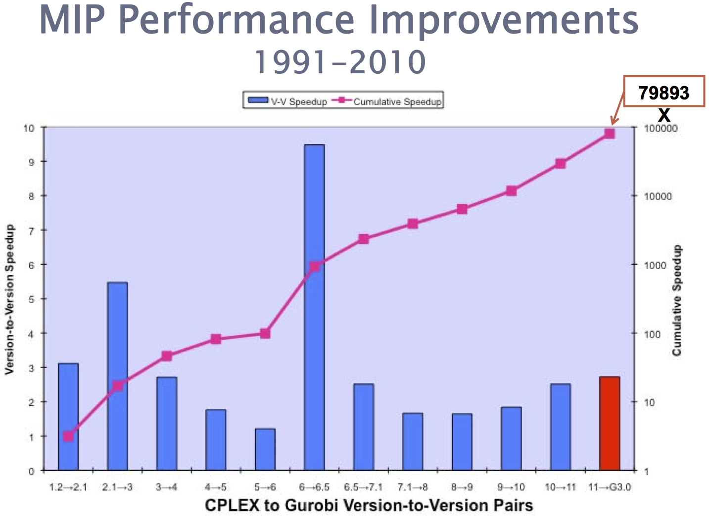
The introduction of Mixed Integer Gomory cuts in CPLEX was The major breakthrough of CPLEX 6.5 and produced the version-to-version speed-up given by the blue bars in the chart below (source: Bixby’s slides available on the web):

Gomory cuts are still subject of research, since they pose a number of implementation challenges. These cuts suffer from severe numerical issues, mainly because the computation of the inverse matrix requires the division by its determinant.

“In 1959, […] We started to experience the unpredictability of the computational results rather steadily” (Gomory, see [4]).”

A recent paper by Cornuejols, Margot, and Nannicini deals with some of these issues [2].

If you like to learn more about how the basis are computed in the CPLEX LP solver, there is very nice paper by Bixby [3]. The paper explains different approaches to get the first basic feasible solution and gives some hints of the CPLEX implementation of that time, i.e., 1992. Though the paper does not deal with Gomory cuts directly, it is a very pleasant reading.

To conclude, for those of you interested in Optimization Stories there is a nice chapter by G. Cornuejols about the Ongoing Story of Gomory Cuts [4].

References

1. C.H. Papadimitriou, K. Steiglitz. Combinatorial Optimization: Algorithms and Complexity. 1998. [book]

2. G. Cornuejols, F. Margot and G. Nannicini. On the safety of Gomory cut generators. Submitted in 2012. Mathematical Programming Computation, under review. [preprint]

3. R.E. Bixby. Implementing the Simplex Method: The Initial Basis. Journal on Computing vol. 4(3), pages 267–284, 1992. [abstract]

4. G. Cornuejols. The Ongoing Story of Gomory Cuts. Documenta Mathematica - Optimization Stories. Pages 221-226, 2012. [preprint]

Last week, more then 700,000 Italian commuters discovered the importance of Operations Research (OR). Nobody explicitly mentioned OR, but due to a horrible crew schedule of Trenord (a train operator with around 330 trains and 2700 employees), the commuters had a long, long, long nightmare. During the whole week, several trains were cancelled (1375 in total) and most of the trains were delayed. A newspaper wrote that a commuter waiting to go home had the painful record of 11 consecutive trains cancelled. The Italian online edition of Wired has an article about this horrible week. If you want to get an idea of the chaos you can search for “caos tilt software trenord” on google.it.

Trenord officially said that the software that planned the crew schedule is faulty. The software was bought last year from Goal Systems, a Spanish company. Rumors say that Trenord paid the Goal System around 1,500,000 Euro. Likely, the system is not faulty, but it “only” had bad input data.

What newspapers do not write

Before the Goal System, Trenord was using a different software, produced by Management Artificial Intelligence Operations Research srl (MAIOR) that is used by several public transportation companies in Italy, included ATM that operates the subway and buses in Milan. In addition, MAIOR collaborates with the Politecnico di Milano and the University of Pisa to improve continuously its software. Honestly, I am biased, since I collaborate with MAIOR. However, Trenord dismissed the software of MAOIR without any specific complaint, since the management had decided to buy the Goal System software.

Newspapers do not ask the following question:

Why to change a piece of software, if the previous one was working correctly?

In Italy, soccer players have a motto: “squadra che vince non si cambia”. Maybe at Trenord nobody plays soccer.

MAIOR is back

Likely, next week will be better for the 700,000 commuters, since OR experts from MAIOR are traveling to Milan to help Trenord to improve the situation.

Disclaimer (post edited on 18th December 2012)

1. I am a Pavia-Milano commuter disappointed of the chaotic week we had.
2. The information reported in this post were obtained with searches on google.it and published on Italian online magazines.
3. Surely, the Goal System is a piece of software as good as MAIOR software is.
4. This post does not intend to offend anyone.

Today, I share seven challenging MIP instances as .mps files along with the AMPL model and data files I used to generate them. While I like the MIPLIBs, I do prefer problem libraries similar to the CSPLIB where you get both a problem description and a set of data. This allows anyone to try with her new model and/or method.

The MIP instances I propose come from my formulation of the Machine Reassignment Problem proposed for the Roadef Challenge sponsored by Google last year. As I wrote in a previous post, the Challenge had huge instances and a micro time limit of 300 seconds. I said micro because I have in mind exact methods: there is little you can do in 300 seconds when you have a problem with potentially as many as $50000 \times 5000$ binary variables. If you want to use math programming and start with the solution of a linear programming relaxation of the problem, you have to be careful: it might happen that you cannot even solve the LP relaxation at the root node within 300 seconds.

That is why most of the participants tackled the Challenge mainly with heuristic algorithms. The only general purpose solver that qualified for the challenge is Local Solver, which has a nice abstraction (“somehow” similar to AMPL) to well-known local search algorithms and move operators. The Local Solver script used in the qualification phase is available here.

However, in my own opinion, it is interesting to try to solve at least the instances of the qualification phase with Integer Linear Programming (ILP) solvers such as Gurobi and CPLEX. Can these branch-and-cut commercial solvers be competitive on such problems?

Problem Overview

Consider you are given a set of processes $P$, a set of machines $M$, and an initial mapping $\pi$ of each process to a single machine (i.e., $\pi_p = i$ if process $p$ is initially assigned to machine $i$). Each process consumes several resources, e.g., CPU, memory, and bandwidth. In the challenge, some processes were defined to be transient: they consume resources both on the machine where they are initially located, and in the machine they are going to be after the reassignment. The problem asks to find a new assignment of processes to machines that minimizes a rather involved cost function.

A basic ILP model will have a 0-1 variable $x_{pi}$ equals to 1 if you (re)assign process $p$ to machine $i$. The number of processes and the number of machines give a first clue on the size of the problem. The constraints on the resource capacities yield a multi-dimensional knapsack subproblem for each machine. The Machine Reassignment Problem has other constraints (kind of logical 0-1 constraints), but I do not want to bore you here with a full problem description. If you like to see my model, please read the AMPL model file.

A first attempt with Gurobi

In order to convince you that the proposed instances are challenging, I report some computational results.

The table below reports for each instance the best result obtained by the participants of the challenge (second column). The remaining four columns give the upper bound (UB), the lower bound (LB), the number of branch-and-bound nodes, and the computation time in seconds obtained with Gurobi 5.0.1, a timeout of 300 seconds, and the default parameter setting on a rather old desktop (single core, 2Gb of RAM).

Instances a1-1, a1-3, a1-5 are solved to optimality within 300 seconds and hence they are not further considered.

The remaining seven instances are the challenging instances mentioned at the begging of this post. The instances a2-x are embarrassing: they have an UB that is far away from both the best known UB and the computed LB. Specifically, look at the instance a2-1: the best result of the challenge has value 198, Gurobi (using my model) finds a solution with cost 54,350,836: you may agree that this is “slightly” more than 198. At the same time the LB is only 110.

Note that for all the a2-x instances the number of branch-and-bound nodes is zero. After 300 seconds the solver is still at the root node trying to generate cutting planes and/or running their primal heuristics. Using CPLEX 12.5 we got pretty similar results.

This is why I think these instances are challenging for branch-and-cut solvers.

Search Strategies: Feasibility vs Optimality

Commercial solvers have usually a meta-parameter that controls the search focus by setting other parameters (how they are precisely set is undocumented: do you know more about?). The two basic options of this parameter are (1) to focus on looking for feasible solution or (2) to focus on proving optimality. The name of this parameter is MipEmphasis in CPLEX and MipFocus in Gurobi. Since the LPs are quite time consuming and after 300 seconds the solver is still at the root node, we can wonder whether generating cuts is of any help on these instances.

If we set the MipFocus to feasibility and we explicitly disable all cut generators, would we get better results?

Look at the table below: the values of the upper bounds of instances a1-2, a1-4, and a2-3 are slightly better than before: this is a good news. However, for instance a2-1 the upper bound is worse, and for the other three instances there is no difference. Moreover, the LBs are always weaker: as expected, there is no free lunch!

If we want to keep a timeout of 300 seconds, there is little we can do, unless we develop an ad-hoc decomposition approach.

Can we improve those results with a branch-and-cut solver using a longer timeout?

Most of the papers that uses branch-and-cut to solve hard problems have a timeout of at least one hour, and they start by running an heuristic for around 5 minutes. Therefore, we can think of using the best results obtained by the participants of the challenge as starting solution.

So, let us make a step backward: we enable all cut generators and we set all parameters at the default value. In addition we set the time limit to one hour. The table below gives the new results. With this setting we are able to “prove” near-optimality of instance a1-2, and we reduce significantly the gap of instance a2-4. However, the solver never improves the primal solutions: this means that we have not improved the results obtained in the qualification phase of the challenge. Note also that the number of nodes explored is still rather small despite the longer timeout.

What if we disable all cuts and set the MipFocus to feasibility again?

With this parameter setting, we improve the UB for 3 instances: a2-1, a2-3, and a2-5. However, the lower bounds are again much weaker. Look at instance a2-1: the lower bound is now 70 while before it was 120. If you look at instance a2-3 you can see that even if we got a better primal solution, the gap is weaker, since the lower bound is worse.

RFC: Any idea?

With the focus on feasibility you get better results, but you might miss the ability to prove optimality. With the focus on optimality you get better lower bounds, but you might not improve the primal bounds.

1) How to balance feasibility with optimality?

To use branch-and-cut solver and to disable cut generators is counterintuitive, but if you do you, you get better primal bounds.

2) Why should I use a branch-and-cut solver then?

Do you have any idea out there?

Minor Remark

While writing this post, we got 3 solutions that are better than those obtained by the participants of the qualification phase: a2-1, a2-3, and a2-5 (the three links give the certificates of the solutions). We are almost there in proving optimality of a2-3, and we get better lower bounds than those published in [1].

References

1. Deepak Mehta, Barry O’Sullivan, Helmut Simonis. Comparing Solution Methods for the Machine Reassignment Problem. In Proc of CP 2012, Québec City, Canada, October 8-12, 2012.

Credits

Thanks to Stefano Coniglio and to Marco Chiarandini for their passionate discussions about the posts in this blog.

Last week in Quebec City, there was the 18th International Conference on Principles and Practice of Constraint Programming. This year the conference had a record of submissions (186 in total) and the program committee made a vey nice job in organizing the plenary sessions and the tutorials. You can find very nice pictures of the conference on Helmut’s web page.

During the conference, the weather outside was pretty cold, but at the conference site the discussions were warm and the presentations were intriguing.

In this post, I share an informal report of the conference as “Je me souviens”.

Challenges in Smart Grids

The invited talks were excellent and my favorite one was given by Miguel F. Anjos on Optimization Challenges in Smart Grid Operations. Miguel is not exactly a CP programmer, he is more on discrete non linear optimization, but his talk was a perfect mixed of applications, modeling, and solution techniques. Please, read and enjoy his slides.

I like to mention just one of his observations. Nowadays, electric cars are becoming more and more present. What would happen when each of us will have an electric car? Likely, during the night, while sleeping, we will connect our car to the grid to recharge the car batteries. This will lead to high variability in night peaks of energy demand.

How to manage these peaks?

Well, what Miguel has reported as a possible challenging option is to think of the collection of cars connected to the grid as a kind of huge battery. This sort of collective battery could be used to better handle the peaks of energy demands. Each car would play the game with a double role: if there is not an energy demand peak, you can recharge the car battery; otherwise, the car battery could be used as a power source and it could supply energy to the grid. This is an oversimplification, but as you can image there would be great challenges and opportunities for any constraint optimizer in terms of modeling and solution techniques.

I am curious to read more about, do you?

Sessions and Talks

This year CP had the thicker conference proceedings, ever. Traditionally, the papers are presented in two parallel sessions. Two is not that much when you think that this year at ISMP there were 40 parallel sessions… but still, you always regret that you could not attend the talk in the other session. Argh!

Here I like to mention just two works. However, the program chair is trying to make all the slides available. Have a look at the program and at the slides: there are many good papers.

In the application track, Deepak Mehta gave a nice talk about a joint work with Barry O’Sullivan and Helmut Simonis on Comparing Solution Methods for the Machine Reassignment Problem, a problem that Google has to solve every day in its data centers and that was the subject of the Google/Roadef Challenge 2012. The true challenge is given by the HUGE size of the instances and the very short timeout (300 seconds). The work presented by Deepak is really interesting and they got excellent results using CP-based Large Neighborhood Search: they classified second at the challenge.

Related to the Machine Reassignment Problem there was a second interesting talk entitled Weibull-based Benchmarks for Bin Packing, by Ignacio Castineiras, Milan De Cauwer and Barry O’Sullivan. They have designed a parametric instance generator for bin packing problems based on the Weibull distribution. Having a parametric generator is crucial to perform exhaustive computational results and to identify those instances that are challenging for a particular solution technique. For instance, they have considered a CP-approach to bin packing problems and they have identified those Weibull shape values that yield challenging instances for such an approach. A nice feature is that their generator is able to create instances similar to those of the Google challenge… I hope they will release their generator soon!

The Doctoral Program

Differently from other conferences (as for instance IPCO), CP gives PhD students the opportunity to present their ongoing work within a Doctoral Program. The sponsors cover part of the costs for attending the conference. During the conference each student has a mentor who is supposed to help him. This year there were around 24 students and only very few of them had a paper accepted at the main conference. This means that without the Doctoral Program, most of these students would not had the opportunity to attend the conference.

Geoffrey Chu awarded the 2012 ACP Doctoral Research Award for his thesis Improving Combinatorial Optimization. To give you an idea about the amount of his contributions, consider that after his thesis presentation, someone in the audience asked:

“And you got only one PhD for all this work?”

Chapeau! Among other things, Chu has implemented Chuffed one of the most efficient CP solver that uses lazy clause generation and that ranked very well at the last MiniZinc Challenge, even if it was not one of the official competitors.

For the record, the winner of the MiniZinc challenge of this year is (again) the Gecode team. Congratulations!

Next Year

Next year CP will be held in Sweden, at Uppsala University on 16-20 September 2013. Will you be there? I hope so…

In the meantime, if you were at the conference, which was your favorite talk and/or paper?

Here we go, my first blog entry, ever. Let’s start with two short quizzes.

1. The well known Dijkstra’s algorithm is:
[a] A greedy algorithm
[b] A dynamic programming algorithm
[c] A primal-dual algorithm
[d] It was discovered by Dantzig

2. Which is the best C++ implementation of Dijkstra’s algorithm among the following?
[a] The Boost Graph Library (BGL)
[b] The COIN-OR Lemon Graph Library
[c] The Google OrTools
[d] Hei dude! We can do better!!!

What is your answer for the first question? … well, the answers are all correct! And for the second question? To know the correct answer, sorry, you have to read this post to the end…

If you are curious to learn more about the classification of the Dijkstra’s algorithm proposed in the first three answers, please consider reading [1] and [2]. Honestly, I did not know that the algorithm was independently discovered by Dantzig [3] as a special case of Linear Programming. However, Dantzig is credited for the first version of the bidirectional Dijkstra’s algorithm (should we called it Dantzig’s algorithm?), which is nowadays the best performing algorithm on general graphs. The bidirectional Dijkstra’s algorithm is used as benchmark to measure the speed-up of modern specialized shortest path algorithms for road networks [4,5], those algorithms that are implemented, for instance, in our GPS navigation systems, in yours smartphones (I don’t have one, argh!), in Google Maps Directions, and Microsoft Bing Maps.

Why a first blog entry on Dijkstra’s algorithm? That’s simple.

• Have you ever implemented an efficient version of this well-known and widely studied algorithm?
• Have you ever used the version that is implemented in well-reputed graph libraries, such as, the Boost Graph Library (BGL), the COIN-OR Lemon, and/or Google OrTools?

I did while programming in C++, and I want to share with you my experience.

The Algorithm

The algorithm is quite simple. First partition the nodes of the input graph G=(N,A) in three sets: the sets of (1) scanned, (2) reachable, and (3) unvisited nodes. Every node has a distance label $d_i$ and a predecessor vertex $p_i$. Initially, set the label of the source node $d_s=0$, while set $d_i=+\infty$ for all other nodes. Moreover, the node s is placed in the set of reachable nodes, while all the other nodes are unvisited.

The algorithm proceedes as follows: select a reachable node i with minimum distance label, and move it in the set of scanned nodes, it will be never selected again. For each arc (i,j) in the forward star of node i check if node j has distance label $d_j > d_i + c_{ij}$; if it is the case, update the label $d_j = d_i + c_{ij}$ and the predecessor vertex $p_j=i$. In addition, if the node was unvisited, move it in the set of reachable nodes. If the selected node i is the destination node t, stop the algorithm. Otherwise, continue by selecting the next node i with minimum distance label.

The algorithm stops either when it scans the destination node t or the set of reachable nodes is empty. For the nice properties of the algorithm consult any textbook in computer science or operations research.

At this point it should be clear why Dijkstra’s algorithm is greedy: it always select a reachable node with minimum distance label. It is a dynamic programming algorithm because it maintains the recursive relation $d_j = \min \{d_i + c_{ij} \mid (i,j) \in A \}$ for all $j \in N$. If you are familiar with Linear Programming, you should recognize that the distance labels play the role of dual variable of a flow based formulation of the shortest path problem, and the Dijkstra’s algorithm costructs a primal solution (i.e. a path) that satisfies the dual constraints $d_j - d_i \leq c_{ij}$.

Graphs and Heaps

The algorithm uses two data structures: the input graph G and the set of reachable nodes Q. The graph G can be stored with an adjacency list, but be sure that the arcs are stored in contiguous memory, in order to reduce the chance of cache misses when scanning the forward stars. In my implementation, I have used a std::vector to store the forward star of each node.

The second data structure, the most important, is the priority queue Q. The queue has to support three operations: push, update, and extract-min. The type of priority queue used determines the worst-case complexity of the Dijkstra’s algorithm. Theoretically, the best strongly polynomial worst-case complexity is achieved via a Fibonacci heap. On road networks, the Multi Bucket heap yields a weakly polynomial worst-case complexity that is more efficient in practice [4,5]. Unfortunately, the Fibonacci Heap is a rather complex data structure, and lazy implementations end up in using a simpler Binomial Heap.

The good news is that the Boost Library from version 1.49 has a Heap library. This library contains several type of heaps that share a common interface: d-ary-heap, binomial-heap, fibonacci-heap, pairing-heap, and skew-heap. The worst-case complexity of the basic operations are summarized in a nice table. Contrary to text-books, these heaps are ordered in non increasing order (they are max-heap instead of min-heap), that means that the top of the heap is always the element with highest priority. For implementing Dijkstra, where all arc lengths are non negative, this is not a problem: we can store the elements with the distance changed in sign (sorry for the rough explanation, but if you are really intrested it is better to read directly the source code).

The big advantage of boost::heap is that it allows to program Dijkstra once, and to compile it with different heaps via templates. If you wonder why the Boost Graph Library does not use boost::heap, well, the reason is that BGL was implemented a few years ago, while boost::heap appeared this year.

Benchmarking on Road Networks

Here is the point that maybe interests you the most: can we do better than well-reputed C++ graph libraries?

I have tried three graph libraries: Boost Graph Library (BGL) v1.51, COIN-OR Lemon v1.2.3, and Google OrTools cheked out from svn on Sep 7th, 2012. They all have a Dijkstra implementation, even if I don’t know the implementation details. As a plus, the three libraries have python wrappers (but I have not test it). The BGL is a header only library. Lemon came after BGL. BGL, Lemon, and my implementation use (different) Fibonacci Heaps, while I have not clear what type of priority queue is used by OrTools.

Disclaimer: Google OrTools is much more than a graph library: among others, it has a Constraint Programming solver with very nice features for Large Neighborhood Search; however, we are interested here only in its Dijkstra implementation. Constraint Programming will be the subject of another future post.

A few tests on instances taken from the last DIMACS challenge on Shortest Path problems show the pros and cons of each implementation. Three instances are generated using the rand graph generator, while 10 instances are road networks. The test are done on my late 2008 MacBookPro using the apple gcc-4.2 compiler. All the source code, scripts, and even this post text, are available on github.

RAND Graphs

The first test compares the four implementations on 3 graphs with different density d that is the ratio $\frac{2m}{n(n-1)}$. The graphs are:

1. Rand 1: with n=10000, m=100000, d=0.001
2. Rand 2: with n=10000, m=1000000, d=0.01
3. Rand 3: with n=10000, m=10000000, d=0.1

For each graph, 50 queries between different pairs of source and destination nodes are performed. The table below reports the average of query times (total time divided by query numbers). The entries in bold highlight the shortest time per row.

In these tests, it looks like my implementation is the winner… wow! Although, the true winner is the boost::heap library, since the nasty implementation details are delegated to that library.

… but come on! These are artificial graphs: who is really interested in shortest paths on random graphs?

Road Networks

The second test uses road networks that are very sparse graphs. We report only average computation time in seconds over 50 different pair of source-destination nodes. We decided to leave out OrTools since it is not very performing on very sparse graphs.

This table below shows the average query time for the standard implementations that use Fibonacci Heaps.

From this table, BGL and my implementation are equally good, while Lemon comes after. What would happen if we use a diffent type of heap?

This second table shows the average query time for the Lemon graph library with a specialized Binary Heap implementation, and my own implementation with generic 2-Heap and 3-Heap (binary and ternary heaps) and with a Skew Heap. Note that in order to use a different heap I just modify a single line of code.

Mmmm… I am no longer the winner: COIN-OR Lemon is!

This is likely due to the specialized binary heap implementation of the Lemon library. Instead, the boost::heap library has a d-ary-heap, that for d=2 is a generic binary heap.

So what?

Dijkstra’s algorithm is so beatiful because it has the elegance of simplicity.

Using an existing efficient heap data structure, it is easy to implement an “efficient” version of the algorithm.

However, if you have spare time, or you need to solve shortest path problems on a specific type of graphs (e.g., road networks), you might give a try with existing graph libraries, before investing developing time in your own implementation. In addition, be sure to read [4] and the references therein contained.

All the code I have used to write this post is available on github. If you have any comment or criticism, do not hesitate to comment below.

References

1. Pohl, I. Bi-directional and heuristic search in path problems. Department of Computer Science, Stanford University, 1969. [pdf]

2. Sniedovich, M. Dijkstra’s algorithm revisited: the dynamic programming connexion. Control and cybernetics vol. 35(3), pages 599-620, 2006. [pdf]

3. Dantzig, G.B. Linear Programming and Extensions. Princeton University Press, Princeton, NJ, 1962.

4. Delling, D. and Sanders, P. and Schultes, D. and Wagner, D. Engineering route planning algorithms. Algorithmics of large and complex networks Lecture Notes in Computer Science, Volume 5515, pages 117-139, 2009. [doi]

5. Goldberg, A.V. and Harrelson, C. Computing the shortest path: A-star search meets graph theory. Proc. of the sixteenth annual ACM-SIAM symposium on Discrete algorithms, 156-165, 2005. [pdf]